")
")
| Issue |
Climatologie
Volume 15, 2018
|
|
|---|---|---|
| Page(s) | 1 - 21 | |
| DOI | https://doi.org/10.4267/climatologie.1314 | |
| Published online | 3 octobre 2019 | |
Temperature variability between 1951 and 2014 in Germany and associated evolution of apple bloom onset
Variabilité de la température entre 1951 et 2014 en Allemagne associée à l’évolution de la floraison des pommiers
Biogéosciences (UMR 6282), équipe CRC, Université de Bourgogne Franche-Comté, Sciences Gabriel, BP 27877, F21078 Dijon Cedex, France
* Cette adresse e-mail est protégée contre les robots spammeurs. Vous devez activer le JavaScript pour la visualiser.
Abstract
Apple tree bloom onset in Germany has advanced by 2 days/decade in 1951-2014 and by 3 days/decade in 1988-2014, behaving similarly in respect to its evolution since 1951 and its sensitivity to temperature to other species’ phenological spring phases. The evolution however was not linear; by conducting a split moving-window dissimilarity analysis (SMWDA) we were able to detect the “break-period” 1987-1989 which coincides with a breakpoint that has been identified in the phases of the North Atlantic Oscillation (NAO). We observed distinct spatial patterns with apple bloom advancing from southwest to northeast and, most interestingly, a longitudinal gradient in the trend of apple bloom onset revealed by a probabilistic principal components analysis (PPCA). In the period of 1951-2014, plants located in the east displayed a much stronger trend (-16.53 days on average) than those in the western part of the country (-6.74 days on average). This pattern seems to be linked to patterns in temperature which is highly correlated to apple bloom onset (best one predictor model: mean temperature March to May, R2 = 0.82, -6 days/°C): the coldest regions exhibit the strongest warming trends and the greatest advances in apple bloom onset.
Résumé
Les dates de floraison des pommiers en Allemagne ont en moyenne avancé de 2 jours/décade de 1951 à 2014 et de 3 jours/décade de 1988 à 2014, en accord avec l’évolution des phases phénologiques d’autres espèces. Cependant, cette évolution n’a pas été linéaire : en réalisant une analyse de dissimilarité d’une fenêtre glissante fractionnée (SMWDA), nous avons détecté une période de rupture entre 1987 et 1989 qui coïncide avec un point de rupture qui a été identifié dans les phases de l’oscillation nord-atlantique (ONA). Nous avons également pu constater une structuration spatiale : la floraison des pommiers progresse du sud-ouest du pays au nord-est; en termes de variabilité interannuelle des dates de floraison, il existe, superposé à un mode principal commun à l’ensemble du pays, un gradient longitudinal qui a été révélé par une analyse probabiliste en composantes principales (PPCA). Entre 1951 et 2014, la tendance à la précocité est plus marquée à l’est du pays (en moyenne -16,53 jours) qu’à l’ouest (en moyenne -6,74 jours) et la floraison des pommiers est très étroitement liée à la variabilité des températures moyennes de mars à mai (R2 = 0,82; -6 jours/°C). Les régions les plus froides montrent les tendances les plus importantes au réchauffement et à la précocité de la floraison.
Key words: Phenology / Germany / climate change / apple bloom / breakpoint
Mots clés : Phénologie / Allemagne / changement climatique / floraison des pommiers / point de rupture
© Association internationale de climatologie 2018
 This is an Open Access article distributed under the terms of the Creative Commons Attribution License CC-BY-NC (http://creativecommons.org/licenses/by-nc/4.0), which permits unrestricted use, distribution, and reproduction in any medium, except for commercial purposes, provided the original work is properly cited.
Introduction
Tree phenology is in general affected by three parameters: photoperiod (day length relative to night length), winter chilling, and temperature. Short photoperiod in autumn and low temperatures induce endodormancy, a state in which all growth in the plant ceases. In this state, no growth will take place even if temperatures are high enough. Since photoperiod in autumn (inducing dormancy) and in spring (release of dormancy) is similar in length, additional information is necessary for the plant to break dormancy: winter chilling. After a certain amount of chilling units (hours spent at low temperatures) have been accumulated and the plant is exposed to short photoperiod, it enters into ecodormancy. Growth is possible in this state, but only if environmental conditions are favourable. In this phase, bud break and afterwards flowering depend on temperatures (Kwolek and Woolhouse, 1982; Li et al., 2003; Heide, 2008). Plants are cold hardy and can tolerate very low temperatures during endodormancy, whereas they can be affected by cold spells in spring if the chilling requirement is already fulfilled and they have reached the state of ecodormancy (Anderson et al., 2010). However, not all woody plants are sensitive to photoperiod. Tropical trees and opportunistic, pioneer species, such as hazelnut, beech and poplar, only rely on temperature information to induce and release dormancy (Körner and Basler, 2010). Heide and Prestrud (2005) showed that apple trees are also part of the plant group that are non-photosensitive and for which temperature is the most deciding factor.
All scenarios of the International Panel on Climate Change (IPCC) anticipate globally increasing temperatures within the next century; the most pessimistic scenario predicts an increase of 3.7 ± 1.1°C, and the most optimistic scenario predicts an increase of 1 ± 0.7°C by 2100 (IPCC, 2014). Effects of global warming on ecosystems and communities and on the phenology of plants and animals in particular have been observed already (Walther et al., 2002; Badeck et al., 2004). These effects are not homogeneous. Several studies have shown that the growing season is lengthening in Western and Central Europe since dormancy induction in autumn is delayed while bud break takes place earlier in spring (Chmielewski and Rötzer, 2002; Menzel et al., 2006). In Eastern Europe, however, the beginning of the flowering season was delayed by two weeks in the period of 1951 until 1998 (Ahas et al., 2002).
In Germany, spring phenological stages across several plant species have advanced and this advancement is well correlated with the air temperature of the preceding months (Menzel, 2003; Englert et al., 2008). Phenological events in temperate regions largely depend on temperatures which are correlated to the North Atlantic Oscillation (NAO, cf. Menzel, 2003). Many studies have found there to be a breakpoint in the phases in the NAO in the second half of the 1980s (see for example Hurrel, 1995; Werner et al., 2000; Scheifinger et al., 2002; Mariani et al., 2012 and Richard et al., 2014). Given the relations between NAO, temperature in Europe and phenological events, it seems likely that the breakpoint in the phases of the NAO be reflected in phenological events.
To test this hypothesis, we analyse in the present study the evolution of the apple bloom onset in Germany since 1951 in detail, examining spatial, temporal and spatio-temporal effects. We then relate apple bloom onset to temperature variability in the same period to analyse whether apple bloom onset has been modified in response to changes in the phases of the NAO and in response to climate change. This study complements that of Chmielewski et al. (2011) which defined phenological models of apple blossom in Germany, but was restricted to the period 1961-2005 and did not examine trends and breakpoints.
With our analyses we want to answer the following questions: (1) Does the date of apple bloom onset in Germany change in the period of 1951 to 2014? (2) Can breakpoints in the study period be observed that mark a change in the temporal development? (3) Which air temperature variables and which period of the year explain apple bloom the best? And (4): Is the evolution of apple bloom onset spatially homogeneous or do spatial patterns in the temporal development exist? How does temperature variability relate to this evolution?
1. Data and methods
1.1. Phenological data set
The German meteorological service (Deutscher Wetterdienst, DWD) has developed a large database of different phenological stages of different plant species that reaches back to the early 20th century. This database (available via the Climate Data Center (CDC) of the DWD, https://opendata.dwd.de/climate_environment/CDC/observations_germany/) is being sustained by volunteers who report the entry of a certain species into a phenological stage in their region, which is associated with an individual stations number, either immediately (immediate reporters) or annually (annual reporters). The volunteers follow a specific protocol (available at https://www.dwd.de/DE/klimaumwelt/klimaueberwachung/phaenologie/daten_deutschland/beobachtersuche/beobachteranleitung.html). The data is quality controlled by the DWD who estimates that 1 to 2% of observations are erroneous each year.
Our dataset comprised both observations from immediate and annual reporters (DWD CDC, 2018b and DWD CDC, 2018c) and we focused our analysis on the onset of bloom of apple trees, i.e. where at least three flowers of a tree are completely open (BBCH code 60), one of the phenological stages that has been observed the longest by the DWD. We did not focus on a specific cultivar of apple trees; instead we used a database with a variety of them. The DWD distinguishes only since 1990 between early and late cultivars. As we were interested in the long term evolution of apple bloom onset, with particular focus on the late 1980s, we chose to use a compiled database with data since 1951. It is important to note that there are disparities in phenological behaviour amongst varieties and that our analysis should therefore be seen as a mean indication for apple trees in general. However, the differences in the beginning of apple blossom between the cultivars are relatively small in Germany (Chmielewski et al., 2011). In addition to the data control of the DWD, we performed a quality control for each station individually using the method of Tukey’s fences (Tukey, 1977), where a value x is considered an outlier if:
![Mathematical equation: $$ \begin{array}{c}x\enspace \notin \enspace \left[{Q}_1-\enspace k*\left({Q}_3-{Q}_1\right),\enspace {Q}_3+k*\left({Q}_3-{Q}_1\right)\right]\\ wh{ere}\enspace k\enspace =\enspace 1.5,\enspace Q1\enspace =\enspace 1{st}\enspace {quartile}\enspace {and}\enspace Q3\enspace =\enspace 3{rd}\enspace {quartile}.\end{array} $$](/articles/climat/full_html/2018/01/climat201815p1/climat201815p1-eq1.gif)
Since phenological data was not continuous for all stations, we reduced the dataset for the spatio-temporal and spatial analyses by excluding stations which had more than 5% of missing values since 1951. The period before 1951 was not analysed since there were less than 32 observations per year. This resulted in a dataset of 54 stations with nearly continuous data between 1951 and 2014 (referred to as “reduced dataset” below, figure 1a).
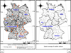 |
Figure 1 (A) Spatial coverage of phenology stations and (B) of weather stations in Germany. The 54 selected phenological stations for the spatio-temporal and spatial analyses are shown in red in Fig. 1a. (A) Réseaux des stations phénologiques et (B) des stations météorologiques en Allemagne. Les 54 stations phénologiques qui ont été choisies pour les analyses spatio-temporelles et spatiales sont montrées en rouge (Fig. 1a). |
Concerning the temporal analysis, the discontinuity of data was not of major importance since the analysis was carried out on the national scale. Despite a strong reduction in observations after 1990, our analyses are robust since the distribution of observation stations stayed fairly homogenous across the country. Therefore we used the whole dataset to calculate national means per year, with as many as 3350 observations in 1980 and as little as 330 observations in 1991.
The whole phenological dataset covers the country nearly uniformly; latitude and longitude distributions of available stations follow Gaussian distributions. 44% of the stations were situated at less than 150m of altitude, 22% between 150 and 300m and 18% between 300 and 450m. In total, 84% of the stations were situated at altitudes of less than 450m which corresponds to the topography of the country since only a little part of it (mainly in the south) is situated at high altitudes. The reduced dataset, which was used for the spatio-temporal and spatial analyses, shows a different geographical distribution. Available stations were concentrated in the south and to the east which is the reason for a different altitude distribution: 26% of the 54 stations were located below 150m of altitude, 20% were situated between 150 and 300m and 26% between 300 and 450m. Therefore, 72% of the stations were located below 450m, compared to 84% for the whole dataset.
1.2. Climate data set
Daily mean temperature data of the period of October 1950 until June 2014 was also obtained via the Climate Data Center of the DWD (DWD CDC, 2018a). It is important to note that the measuring standards were not the same in East and West Germany before the reunification of the country in 1989 when they were harmonised, however there were manual quality controls. In order to minimize error sources in our analyses, we used the same method as for the phenological data set to remove outliers. Since we were also interested in the spatial aspect of the connection between air temperature and apple bloom evolution, we chose to use station temperature data.
Similarly to the phenological dataset, there is a discontinuity in station data concerning the daily temperatures. Nevertheless, we deemed the dataset large enough to calculate representative daily temperature mean values on the national level. These were calculated using data from at least 386 stations spread over the country (figure 1b). With the obtained daily mean temperatures, we were able to calculate several seasonal and bi-monthly means for each year of the study period. Both phenological and climate data that we used is available at the Climate Data Center of the DWD (https://opendata.dwd.de/climate_environment/CDC/).
1.3. Statistics
1.3.1. Spatio-temporal analysis of apple bloom onset
We used a split moving-window dissimilarity analysis (SMWDA) with Monte-Carlo significance on the complete dataset (Kemp et al., 1994; Bigot et al., 1998) employing four different window sizes (10, 16, 22 and 26 years) in order to find out whether breakpoints could be determined in the evolution of the apple bloom trend between 1951 and 2014. This method places a window divided in two subparts at the beginning of a data series. Then, the mean values of the two subperiods and the Euclidian distance between the two of them are calculated, and the window is moved forward using a one-year step. Subsequently, the distance values are plotted against the location of the window midpoint where peaks correspond to potential discontinuities in the time series. To determine the significance of the breakpoints, a Monte Carlo test is applied where the individual data points are redistributed randomly and a test statistic is created with the mean distances. Then, we fitted linear regressions on the time series of mean apple bloom onset for the individual periods limited by the calculated breakpoints. Linear regressions were also fitted to the full time series (1951-2014) to detect long-term trends.
To see whether the results of the analyses of the complete dataset held true when analysing the reduced dataset of 54 stations, we repeated the SMWDA on the averaged bloom dates of the 54 stations in the period of 1951 to 2014. Subsequently, we analysed spatial patterns of the mean apple bloom date from 1951 to 2014 for the reduced dataset by conducting stepwise forward multiple regression (with the criterion to include variables if p < 0.05) taking the variables latitude, longitude and altitude into account. We also examined the relationship between spatial variables and the trend of bloom at the individual stations to see whether it was determined by spatial patterns.
We then performed a probabilistic principal component analysis (PPCA) to analyse whether a covariance in time of the 54 stations existed. This method allows performing a PCA on a dataset with missing values, which can be reconstructed afterward. It is based on the application of an expectation-maximization algorithm on PCA where maximum likelihood values for missing data are directly estimated at every iteration (Roweis, 1998). This method, proposed by Roweis (1998), was further simplified by Verbeek et al. (2002). PPCA was successfully used in several climatological studies at interannual time-scales, either to reconstruct data matrices (e.g. Moron et al., 2016) or to analyse the space-time variability of climate variables (e.g. Lopes et al., 2016). In our study, PPCA was applied to the interannual variations of the apple bloom dates at the 54 stations.
1.3.2. Climate variables explaining temporal variability of apple bloom onset
Previous studies that have analysed the relation between phenology and temperature used 2- or 3-monthly mean spring air temperature as a predictor for bloom onset (cf. Menzel, 2003; Chmielewski et al., 2004). However, models of bloom prediction often use sequential models in which not only spring temperature but also winter temperature is included in order to account for the chilling effect, see for example Legave et al. (2008) In these models, cumulated temperatures are used since plant development and growth do not occur below a certain threshold just as the chilling requirement is not fulfilled if temperatures are too high; mean temperatures might not be a satisfactory variable in this case. However, it is very difficult to put numbers to these thresholds since they may vary between species.
Therefore, we calculated running correlations over 2-month periods of different temperature variables with the onset of apple bloom in Germany to determine which periods and which kinds of thermal variables explained the onset of apple bloom the best. We calculated temperature means as well as positive cumulated temperatures representing the heating effect and negative cumulated temperatures representing the chilling effect. We used two different ways to calculate the cumulated temperatures (after Legave et al., 2013):
 (eq. 1)
 (eq. 2)

Firstly, we used a linear model, i.e. we added up all temperatures below or above 7°C (as described in equation 1). This threshold was chosen following Naor et al. (2003) and Ferree and Warrington (2003) in Celton et al. (2011). Secondly, we used an exponential model (equation 2) to include the possible scenario that temperatures well above 7°C promote growth and development better than temperatures just above the threshold. We then calculated running correlations between the five temperature variables: mean temperature, linearly cumulated positive temperature (eq. 1b), linearly cumulated negative temperature (eq. 1a), exponentially cumulated positive temperature (eq. 2b), exponentially cumulated negative temperature (eq. 2a) and the onset of apple bloom (using the averaged date per year of the whole dataset), starting October 1st and moving the correlation window by one week per iteration. As a result we obtained correlations of 31 different periods of the year for five different temperature variables.
Subsequently, we did several stepwise forward multiple regressions, including only time periods of variables for which the initial correlation was significant (p-value < 0.05) and only one prediction period per variable for every model (to avoid using one variable twice in a model). Two further stipulations were that the starting date of the prediction period of the cumulated positive temperatures had to be after January 1st (since they were supposed to simulate the warming effect), and that the starting date of the cumulated negative temperatures had to lie in the previous year (to take the chilling effect into account). This way, we obtained for each possible combination meeting the stipulations the best model. Out of these best models, we chose those where R2 > 0.9. We then examined which temperature variable and which time period for each variable was used the most to create a “best model”.
1.3.3. Spatial temperature analysis and relations with apple bloom onset
In order to conduct a spatial analysis of temperatures and apple bloom onset we had to match climate stations to phenological ones. To increase representativeness and to cover the whole period of 1951 to 2014, we averaged daily temperatures of all climate stations that were in the vicinity of a phenological station, i.e. not further away than 0.32° in latitude and 0.52° in longitude (about 35 km). An additional criterion was that the elevation of the climate stations should not differ by more than 60 m from that of the phenological station, except for three stations where we increased this criterion to include stations that were up to 100 m lower than the phenological station. Using these criteria, we had to decrease the dataset of 54 stations to 50 stations since there was not sufficient data available for four of them. For these 50 stations we calculated mean air temperatures and temperature trends between 1951 and 2014 for two different seasonal periods: November 25th to January 24th and February 10th to May 2nd because these periods will show to exert control on apple bloom.
Analogous to the spatial analysis of the apple bloom onset, we used stepwise forward regression to analyse the relationship between the spatial variables (latitude, longitude and altitude) and the mean temperatures and temperature trends. We also calculated Pearson correlation coefficients for the individual variables. We furthermore analysed the relation between the spatial pattern of temperature trend and mean temperature using Pearson’s correlation coefficient. To see to which extent apple bloom trends are linked to temperature means and trends, we conducted linear regressions between apple bloom trends and mean temperatures in spring and winter as well as between apple bloom trends and temperature trends in spring and winter.
2. Results
2.1. Spatio-temporal analysis of apple bloom onset
On average, apple bloom onset in Germany in the period of 1951 to 2014 was on May 2nd, with a relatively low interannual variability of one week (figure 2a).
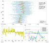 |
Figure 2 Evolution of the apple bloom onset in Germany between 1951 and 2014, at all available phenological stations (Fig. 2a, dots) and as an average over Germany (Fig. 2a, solid line), and results of a split moving-window dissimilarity analysis (SMWDA, Fig. 2b and 2c). The SMWDA, where 4 different window sizes were chosen: 10, 16, 22 and 26 years, revealed a breakpoint in the period of 1987 until 1989, which is reflected in the two different trend lines (in green) in 2a. Evolution de la floraison des pommiers en Allemagne entre 1951 et 2014 de toutes les stations disponibles (points, Fig. 2a) et de la moyenne en Allemagne (ligne solide, Fig. 2a), et résultats d’une analyse de dissimilarité d’une fenêtre glissante fractionnée (SMWDA, Fig. 2b et 2c). La SMWDA, où 4 tailles de fenêtre différentes ont été utilisées : 10, 16, 22 et 26 années, a révélé un point de rupture dans la période 1987-1989 montré avec les deux courbes de tendance différentes (en vert) dans la Fig. 2a. |
A linear regression fitted over the whole period gave a significant negative trend of -0.22 days/year (p-value < 0.001), suggesting a gradually earlier apple bloom onset. However, the SMWDA conducted on the whole dataset revealed breakpoints at the end of the 1980s (in the years 1987-1989). These breakpoints are very robust since they held true for all window sizes used in the analysis (figure 2c). The two sub-periods before and after this breakpoint actually show contrasted behaviours. A regression over the years 1951 to 1988 showed a significant trend towards a later bloom (+0.17 days/year = 1.7 days/decade, p-value < 0.1). Only the trend in the second part of the study period was negative (-0.30 days/year on average = -3 days/decade, p-value < 0.05). When comparing the two subperiods, the mean apple bloom onset in the period 1988 to 2014 was about ten days earlier than in the first subperiod (May 6th in the first period compared to April 26th in the second period).
When examining the spatial patterns of the mean apple bloom date, we found it to be strongly determined by latitude, longitude and altitude (table 1 and figure 3a). A model taking these three variables into account explained 83% (adjusted R2) of the variability of the apple bloom in the dataset of 54 stations in Germany. The higher the latitude and altitude and the further east in the country, the later the apple bloom, i.e. apple bloom in Germany occurs earlier in the southwest than in the northeast of the country and earlier at lower altitude than at higher altitude. The only significant spatial variable related to the apple bloom trend was longitude (table 1). The further east one goes, the stronger the trend to an earlier date of bloom (figure 3b).
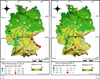 |
Figure 3 A) Mean flowering date (days of year from 1st January) and B) linear trend (number of days in 64 years) of flowering date of apple trees at 54 stations in Germany 1951-2014. Date moyenne (jours à partir du 1 janvier, Fig. 3a) et tendance linéaire (nombre de jours en 64 années, Fig. 3b) de la floraison des pommiers pour 54 stations en Allemagne de 1951 à 2014. |
Spatial analysis of mean apple bloom onset (a) and apple bloom trend (b) in Germany between 1951 and 2014. The results refer to a multiple linear regression in (a) and a simple linear regression in (b); 54 stations were analysed. Analyse spatiale de la floraison moyenne des pommiers (a) et de la tendance de la floraison (b) en Allemagne entre 1951 et 2014. Les résultats se réfèrent à une régression multiple linéaire (a) et à une simple régression linéaire (b); 54 stations ont été analysées.
As a mean to synthesize the spatial patterns of interannual variations in apple bloom dates, PPCA was applied to the matrix of 64 years and 54 stations. Note that we checked that in this reduced data set breakpoints and trends were consistent with those obtained with the full data set. The first two principal components, which together explain 79% of the variance, were retained. All 54 stations were highly correlated (Pearson correlation coefficient > 0.7) with PC1 which represented 75% of the information (results not shown). The corresponding time series (figures 4a and 4b) show a very similar temporal variation as found above from the complete data set. The same breakpoints (or “break period”) as identified above (1987 to 1989) were found on the PC1 times series. PC1 therefore confirms that there is a strong, quasi-uniform signal of apple bloom variability across the whole of Germany. Only 19 stations were significantly correlated to the second principal component (PC2, which represented 4% of the total information). The stations that showed the lowest correlations with PC1 showed the highest correlations with PC2 and were situated in the eastern part of Germany (figure 4c). The corresponding time-series (figure 4b) showed a linearly advancing date of bloom without breakpoint. On the whole, the PPCA revealed that all stations followed the same trend towards an earlier bloom date despite a great interannual variability but that there were 19 stations that behaved slightly differently, as demonstrated by PC2 which superimposed on the PC1 signal at these stations.
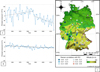 |
Figure 4 Results of a probabilistic principal component analysis (PPCA) of the evolution of the apple bloom onset between 1951 and 2014 at 54 stations in Germany. Fig. 4a and 4b: time-series of the first two principal components (PC1 and PC2). A split moving-window dissimilarity analysis (SMWDA) of the time series of PC1 revealed a breakpoint in the period of 1987-1989. The trends as indicated by the dotted and solid lines are significant at a level of 0.05. Fig. 4c shows Pearson correlation coefficients of the time series of the individual stations with PC2. Solid circles show a correlation where p-value < 0.001, and broken circles show a correlation where 0.001 < p-value < 0.1. The principal components are expressed in the unities of the original variables (days) and take the variance associated with each component into account. Résultats d’une analyse probabiliste en composantes principales (PPCA). Fig. 4a et 4b : séries temporelles des deux premières composantes (PC1 et PC2). Une analyse de dissimilarité d’une fenêtre glissante fractionnée (SMWDA) de la série chronologique PC1 a révélé un point de rupture dans la période de 1987 à 1989. Les tendances (indiquées par les traits pointillés et le trait continu) sont significatives au niveau de 0,05. La carte à droite (Fig. 4c) montre les coefficients de corrélation de Pearson des séries chronologiques des stations individuelles avec PC2. Des cercles continus montrent une corrélation avec une p-value < 0,001 et les cercles interrompus montrent une corrélation avec 0,001 < p-value < 0,1. Les composantes principales sont exprimées dans les unités des variables de départ (jours) et tiennent donc compte de la variance associée à chaque composante. |
To further examine the stations where a significant correlation (p-value < 0.1) with PC2 was found, we divided them into two groups (group 1: negative correlation with PC2, group 2: positive correlation with PC2). We then performed an analysis of variance (ANOVA) on the means and trends of these two groups to see whether the mean bloom date and the trend of the bloom date of the stations that showed a positive correlation to PC2 differed significantly from those that showed a negative correlation. We furthermore fitted linear regressions over the mean bloom dates of each group in the period 1951 to 2014 to examine if the evolution of the bloom date over time was the same for the two groups.
The ANOVAs performed on the two groups showed that yearly mean bloom dates and trends of bloom dates differed significantly (mean: F1, 127 = 58, p-value < 0.001; trend: F1, 18 = 44, p-value < 0.001), with stations of group 1 (negative correlations with PC2) blooming earlier on average and displaying a weaker trend of an advancement of bloom. The stations belonging to group 1 were situated in the western part of the country and showed a significant trend towards a later date of bloom in the period before the breakpoint in 1988 while this trend was reversed in the second period, whereas the stations in group 2 showed no trend in 1951-1988 but a negative trend in 1988-2014 (table 2 & figure 5). Group 1 displayed a trend of -6.74 days on average in the period of 1951 to 2014, while group 2 displayed an average trend of -16.53 days in the same period. Overall, it was noted that in the period of 1951 to 1988 the difference in the mean bloom dates between the two groups was decreasing with time while it stayed approximately the same since 1988. Altogether, while significant regional differences are present, they are only superimposing the overall signal of a significantly earlier bloom.
 |
Figure 5 Time series of spatially-averaged bloom dates of two different groups of stations: group 1 including 10 stations (out of 54 stations analysed) that have a negative correlation with PC2 (in blue) and group 2 including 9 stations that have a positive correlation with PC2 (in red). Significant trends (p-value < 0.05) are indicated by dotted lines. Séries chronologiques de deux groupes de stations différents : groupe 1 qui rassemble les stations qui ont une corrélation négative avec PC2 (10 des 54 stations analysées) et groupe 2 qui consiste en 9 stations ayant une corrélation positive avec PC2. Des tendances significatives (p-value < 0,05) sont indiquées avec des lignes en pointillés. |
Slopes of linear regressions of the mean apple bloom onset of two subgroups, for the whole time period and for the two subperiods as defined from the split moving-window dissimilarity analysis (SMWDA). n.s.: not significant, *: 0.01 < p-value < 0.05, **: 0.001 < p-value < 0.01, ***: p-value < 0.001. Pentes des régressions linéaires de la floraison moyenne des pommiers de deux sous-groupes, sur la période entière et sur les deux sous-périodes comme définies par l’analyse de dissimilarité d’une fenêtre glissante fractionnée (SMWDA). n.s. : pas significatif, * : 0.01 < p-value < 0.05, ** : 0.001 < p-value < 0.01, *** : p-value < 0.001.
2.2. Climate variables explaining temporal variability of apple bloom onset
All temperature variables that we chose to analyse were very well correlated to the onset of apple bloom averaged over Germany as a whole, with the best predictive time period for all variables being the two months starting from the beginning of March (correlations around -0.8 and +0.7 for the different variables, figure 6).
 |
Figure 6 Running correlations between apple bloom onset dates averaged over Germany and 5 different temperature variables. The 5 different variables were each calculated over a 2-month period starting from the day indicated by the individual points (e.g. the points corresponding to October 1st indicate correlations with variables that were calculated over the period October 1st – November 30th). “cum pos lin” stands for linearly cumulated positive temperatures (> 7°C, eq. 1b), “cum neg lin” for linearly cumulated negative temperatures (< 7°C, eq. 1a), “cum pos exp” for exponentially cumulated positive temperatures (eq. 2b) and “cum neg exp” for exponentially cumulated negative temperatures (eq. 2a). Corrélation glissante entre la date de floraison moyenne des pommiers en Allemagne et 5 variables de température différentes. Les 5 variables ont été calculées sur une période de deux mois, le premier jour de cette période est indiqué par les points sur le graphique (par exemple, les points correspondant au 1 octobre indiquent des corrélations avec des variables qui ont été calculées sur la période 1 octobre – 30 novembre). « cum pos lin » signifie température cumulée positive linéaire (> 7°C, éq. 1b), « cum neg lin » signifie température cumulée négative linéaire (< 7°C, éq. 1a), « cum pos exp » signifie température cumulée positive (éq. 2b) et « cum neg exp » température cumulée négative exponentielle (éq. 2a). |
Negative correlations with mean temperature and the cumulated positive temperature variables as well as positive correlations with the cumulated negative temperature variables indicate that the colder this period, the later the flowering. Correlations slowly decrease to about zero when considering temperature during gradually earlier periods, from February back to November. The best one-predictor model included the 2-month mean temperature starting March 10th and explained 82% of the observed variance in apple bloom onset (p-value < 0.001, figure 7). A change of 1°C in the mean temperature from mid-March to mid-May equals an advancement of bloom onset of approximately 6 days.
 |
Figure 7 Relation between bloom onset dates averaged over Germany and mean temperature in the period between 10th March and 10th May (best one-predictor model). The chosen temperature variable explains 82% of the variance in a linear regression. The points represent the years 1951 to 2014. Relation entre le début moyen de la floraison en Allemagne et la température moyenne entre le 10 mars et le 10 mai (meilleur modèle avec un prédicteur). La variable de température choisie explique 82% de la variance dans une régression linéaire. Les points représentent les années 1951 à 2014. |
As a second step we carried out many multiple regressions of the different time periods in an attempt to increase the explanatory power of the model. The time period of the variable mean temperature that was used the most started on February 10th. The most often used variable in the 909 best models (where R2 > 0.9) was the linear cumulated positive temperature, followed by mean temperature and exponential cumulated positive temperature. Exponential cumulated negative temperature was used more often than linear cumulated negative temperature. Since we only wished to have one predictor for the chilling effect and one for the heating effect, we only used one of the negative/positive cumulated temperature variables. Altogether, the best model (with starting day of time period over which the temperature variable was calculated in subscripts) included the two month mean temperature10/02, linear cumulated positive temperature03/03 and exponential cumulated negative temperature25/11 (table 3). This model explained 91% of the variance in apple bloom onset.
Best model of temperature variables explaining the onset of apple bloom. The model included three different variables and explained 91% of the variance. Meilleur modèle des variables de température expliquant le début de la floraison des pommiers. Ce modèle comprend trois variables différentes et explique 91% de la variance.
In order to assess whether the trends and breakpoints found in the phenological data were related to changes in any of the explanatory climate variables, we next analysed the temporal variations of the latter. Since the mean temperature10/02 and linear cumulated temperature03/03 were not well enough correlated, we analysed the evolution of the temperature variables separately conducting SMWDA, linear regression and ANOVA. We only found breakpoints in the mean temperature10/02 variable. All four window sizes of the SMWDA showed breakpoints between 1987 and 1989, consistent with the ones found in apple bloom onset. It is to note that even though the trend in the mean temperature10/02 of the overall period 1951-2014 was significant (+0.03°C/year, p-value < 0.05), there were no significant trends of the two periods divided by the breakpoint (figure 8). However, the mean temperatures10/02 of the two periods were significantly different (as tested by an ANOVA, F1, 63 = 10.64, p-value < 0.01). In the period of 1951 to 1988 the mean temperature10/02 was at 2.78°C while it was at 4.47°C in the period of 1988 to 2014.
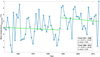 |
Figure 8 Yearly spring mean temperatures (mean of 10th February until 10th April) in Germany between 1951 and 2014. The SMWDA revealed breakpoints in the years 1987 to 1989, but the two periods divided by the breakpoint (1951-1988 and 1988-2014) do not show significant trends. The spring mean temperature of the two different periods is significantly different (ANOVA: F1, 63 = 10.64, p-value < 0.01). In the period of 1951 to 1988 spring mean temperature was at 2.78°C while it was at 4.47°C in the period of 1988 to 2014. The overall trend is significant with an increase in temperature of 0.03°C/year (p-value < 0.05). Températures annuelles moyennes du printemps (moyenne du 10 février au 10 avril) en Allemagne entre 1951 et 2014. La SMWDA révèle des points de rupture entre 1987 et 1989, mais il n’y a pas de tendances significatives dans les deux périodes divisées par ces points de rupture (1951-1988 et 1988-2014). La température moyenne des deux périodes différentes diffère de façon significative (ANOVA : F1, 63= 10,64, p-value < 0.01). Sur la période de 1951 à 1988, la température moyenne était de 2,78°C tandis qu’elle était de 4,47°C sur la période 1988-2014. La tendance globale est significative avec une augmentation de 0,03°C/année (p-value < 0,05). |
Besides mean temperature10/02, only linear cumulated positive temperature03/03 showed a significant trend. Mean temperatures of the winter period (25/11 – 24/01) evolved towards higher temperatures, whereas no significant trend was found in the evolution of exponential cumulated negative temperatures of the same period (which might be due to the calculations that include an exponential effect of cold spells). This suggests that both the trend and interannual variations of apple bloom onset are related to late winter and spring temperature, while some of the interannual variations of flowering are also explained by the severity of winter, very severe winters inducing a late apple bloom onset.
To see whether the relationship between the different temperature variables and the onset of bloom changed in the two periods before and after the breakpoint, we fitted several linear regressions over the two periods and the whole study period. In none of the variables could a significant change be detected. However, the best predictive time period for the variables changed: in 1988 to 2014 the best predictive time period was approximately one week earlier for all variables than in 1951 to 1988, in good agreement with the one week change in mean apple bloom onset between the two sub-periods.
2.3. Spatial temperature analysis and relations with apple bloom onset
We finally analysed spatial patterns of apple bloom onset and temperatures by examining the geographical variables associated with the temperature indices identified in the previous section as good predictors of apple bloom. The two groups of stations identified by the PPCA showed a significant difference in the spring mean temperature: group 1 (stations situated in the west, and showing a negative correlation to PC2; figure 4c) had a significantly higher spring mean temperature (6.05°C) than the easternmost stations in group 2 (3.65°C): ANOVA, F1, 16 = 31.12, p-value < 0.001.
The multiple stepwise forward regressions showed a surprising result: Winter mean temperatures (November 25th – January 24th) depended on only longitude and altitude (R2 = 0.93, p-value < 0.001), while spring mean temperatures (February 10th – May 2nd, which was the main period included in the multiple regressions) depended also on latitude (R2 = 0.94, p-value < 0.001). Both spring and winter temperature trends were determined by latitude and longitude (R2 = 0.32 and R2 = 0.38, p-values < 0.001): in winter, the strongest trends were registered in the southeast of Germany while the strongest trends in spring were registered in the northeast. Pearson’s correlation coefficient revealed that temperature trends are linked to mean temperatures (winter: R50 stations = -0.52, p-value < 0.001; spring: R50 stations = -0.31, p-value < 0.05): the lower the mean temperature, the stronger the temperature trend towards a warmer spring/winter.
Similarly, the relationships between the spatial patterns of apple bloom trends and temperature were examined. A relation exists between apple bloom trend and mean temperatures in winter and in spring (winter: R = 0.3, p-value < 0.05; spring: R = 0.36, p-value < 0.05) and between apple bloom trend and temperature trends in spring (R = -0.44, p-value < 0.01): the lower the temperatures, the stronger the temperature trend and the stronger the apple bloom trend towards an earlier date of bloom.
3. Discussion
3.1. A breakpoint in the late 1980s marks a change in the temporal development of apple bloom onset
Apple bloom onset in Germany in the period of 1951 to 2014 was on average on May 2nd. Using SMWDA, we found a breakpoint in the evolution in apple bloom onset in the late 1980s. When comparing the two subperiods, the mean apple bloom onset in the period 1988 to 2014 was about ten days earlier than in the first subperiod (May 6th in the first period compared to April 26th in the second period). Over the whole study period we found a significant trend of advance in the apple bloom onset of 0.2 days/year, i.e. 2 days per decade. However, it is crucial to mention that the advance in the second sub-period was 50% greater with an advance of 3 days per decade. Many studies conducted on the subject of phenological events and their relations to temperature provide the classical linear trend model, i.e. a linear trend calculated over the whole study period without testing for breakpoints first (amongst others Menzel et al., 2001; Ahas et al., 2002; Chmielewski et al., 2004; Englert et al., 2008). This makes it difficult to compare our results to the mentioned studies. However, the value of a 2 day advance/decade for apple bloom onset is the same that was found by Menzel et al. (2001) who studied spatial and temporal variability of phenological seasons in Germany in the period of 1951 to 1996, and our results fit well within the ranges mentioned in the other studies where the phenology of other plant species were analysed (cf. Ahas et al., 2002; Englert et al., 2008).
Climate in Europe is strongly influenced by the North Atlantic Oscillation (NAO). Positive phases of the NAO correspond to a very strong Azores high and Icelandic low, and are associated with heavy rainfall and mild weather in northern Europe and in the east of the United States. At the same time, the Mediterranean region may be affected by the Siberian high which leads to colder, drier weather than usual. Negative phases on the other hand are associated with inverse atmospheric conditions and are connected to harsh winters and hot summers, influence of the Siberian high (Barnston and Livezey, 1987). Periodically, the phases of the NAO change. Tomé and Miranda (2005) suggested the years 1968 and 1992 as breakpoints, but several studies have highlighted the change in phase of the NAO that took place in the second half of the 1980s (Hurrel, 1995; Werner et al., 2000; Scheifinger et al., 2002). Mariani et al. (2012) identified in a recent analysis of surface temperature in Europe two sub-periods in the period of 1951 to 2010, with the breakpoint dividing the two being situated in 1987/88. At a regional scale, this breakpoint has also been found in Burgundy (France) by Richard et al. (2014). Since phenological events largely depend on temperature which is correlated to the NAO (cf. Menzel, 2003), those concerning species that are not sensitive to photoperiod even more so, the “break-period” that we found in the apple bloom onset in Germany at the end of the 1980s corresponds well to the findings in the studies cited above.
The effects of the regime shift in the late 1980s have been analysed in several other studies: an upward habitat shift of brown trout populations in Switzerland has been observed (Hari et al., 2006) and the shift has been detected across different trophic levels in the German Bight (Schlüter et al., 2008). Figura et al. (2011) even noted an abrupt increase in Swiss ground water temperatures in 1987 and related this change to a modification in the Arctic Oscillation. Reid et al. (2016) conducted a study in which they analysed regime shifts in the 1980s all over the world. These shifts occurred at slightly different times, the earliest in South America in 1984, in North America and the North Pacific in 1985, in the North Atlantic Ocean in 1986, in Europe in 1987 and in Asia in 1988. They propose that the regime shifts are a result of rapid global warming from anthropogenic and natural forcing, the latter associated with a recovery from the eruption of the El Chichón volcano in Mexico in 1982.
3.2. Apple bloom onset is linked to spring mean temperatures
Our best one-predictor model linking spring mean temperature (mid-March – mid-May) to apple bloom onset revealed that a 1°C increase in spring temperature leads to a 6 day advance in apple bloom. This value corresponds closely to the value of 7 days advance in leaf unfolding for a change of 1°C (February – April) found in a study conducted by Chmielewski and Rötzer (2001) for the period of 1969 to 1998, using four different tree species as a proxy for spring phenology. Our result fits well with the study of Vitasse et al. (2009) as well who found temperature sensitivity for oak to be at -7.26 days/°C (mean temperature January 1st – May 31st) in France. However, -6 days/°C appear to be generous when comparing them to Menzel et al. (2006) who found an average of -2.5 days/°C and a maximum of -4.6 days/°C in spring/summer phenological stages in Germany. This disparity might be due to the different periods of time that were studied (1971 to 2000 in Menzel et al. (2006); 1951-2014 in the present study), or in the species composition on which the results of Menzel et al. (2006) are based, apple trees not being among them.
Opportunistic species that are not sensitive to photoperiod such as the apple tree are tracking the warming pattern of climate change, however late successional species such as oak and beech that are sensitive to photoperiod will very likely exhibit a different behaviour. It might take several centuries for new genotypes to emerge, adapted to a warmer climate (Körner and Basler, 2010). This discrepancy will expose opportunistic species to a higher risk of late frosts while at the same time putting late successional species at a disadvantage in their competitive behaviour. The varying temperature sensitivity in plants also has consequences for interactions with other trophic levels, especially the mutualism with pollinators. Bartomeus et al. (2011) found that pollinator and plant responses to warming climate are similar. Memmott et al. (2007) however show in their study that by doubling the carbon dioxide quantity in the atmosphere a dissymmetry between phenological phases of pollinators and plants might exist where 50% of pollinating activity will take place when plants are not in bloom. Bartomeus et al. (2013) underline the importance of biodiversity: biodiversity-rich communities are more robust and could compensate for single asynchronous species-species relationships. Humans are about to reduce biodiversity at an astonishing pace and are therefore causing ecosystems and communities to be less robust and more vulnerable.
3.3. The evolution of apple bloom onset was not spatially homogeneous: colder (eastern) places displayed a faster upward trend in temperatures and apple bloom consequently displayed a greater advance in bloom
Early on it was discovered that spring phenological phases shift from southwest Europe to northeast Europe (28-50 km/day; Schnelle, 1948). Menzel et al. (2005) confirmed these findings which explain why we found distinct spatial patterns in the mean apple bloom onset. Our latitudinal and longitudinal gradients were lower than what was found in the mentioned study (in this study: a latitudinal gradient of 1.16 days/degree latitude and 0.18 days/degree longitude, compared to 2.18 days/degree latitude and 0.52 days/degree longitude in Menzel et al. (2005)), however, the spatial and temporal scopes of their study were different as well as the species included in their analyses.
A novel result of our study was the observation that colder (eastern) places seem to be more affected by the general warming trend and displayed a faster upward trend in temperatures than warmer (western) places. Since colder places exhibited stronger trends, and apple bloom onset is linked to temperature, apple bloom onset in colder regions consequently also displayed a greater advance in bloom. This observation is supported by the PPCA that highlighted two groups of stations, stations of group 1 situated to the west and stations of group 2 situated to the east. Apple trees in the western part of the country bloomed earlier and displayed a weaker trend of advance (-6.74 days on average in the period of 1951 to 2014) compared to the eastern part of the country; we even detected an evolution towards a later date of bloom in the period before 1988. Apple trees in the eastern part of Germany on contrast bloomed later and displayed a trend more than twice as great with -16.53 days on average in the period of 1951 to 2014. The mean spring temperature in the east was approximately 2.5°C lower than in the west. Of course, these results must be regarded with caution since altogether only 19 stations were contained in the groups determined by the PPCA. The longitudinal gradient explained 13% of the variation in the evolution of the apple bloom onset.
However, it must be taken into account that the stations of the data subset used for the spatio-temporal and spatial analyses showed a different geographical distribution than the whole dataset, with more stations in the reduced dataset situated at higher altitudes. The location of the country itself might also influence the results, especially the calculated gradients, since northern parts of the country are affected by an oceanic climate and the buffer effect of the sea while other (south-eastern) parts are more subject to a continental climate. Lastly, our results are an indication for apple trees in general; it is very likely that intraspecific apple bloom onset variability exists in respect to responses towards a warmer climate because different cultivars exhibit slightly different phenologies.
Conclusion
In the period of 1951 to 2014, apple tree bloom onset in Germany has advanced by 2 days/decade, but by 3 days/decade in the period of 1988 to 2014. This evolution and the temperature sensitivity that we observed (6 days earlier per degree Celsius of the 2 month mean temperature starting on March 10th) are similar to other species’ phenological spring phases that have been studied previously. However, the abrupt shift at the end of the 1980s, characterised by a distinct advance in apple bloom onset and which coincides with a breakpoint in the phase of the North Atlantic Oscillation, has attracted little attention to date. The question remains open how much of the observed variability is natural variability of the NAO that influences weather in Europe, and how much of it can be attributed to human induced climate change. An interesting finding of the study is that the long-term linear trend is not solely explained by the shift in the late 80s, the trend beyond this year is also quite strong, which suggests that the signal of anthropogenic climate change is predominant.
It would be interesting to see whether the NAO regime shift that has been recognized at a larger scale (cf. Reid et al., 2016) can be found in other species’ phenological response in Germany and the surrounding countries, and whether the rate of advancement in phenological spring seasons is similarly high to ours in the second subperiod (-3 days/decade in 1988-2014). It might also be interesting to consider other phenological seasons since it has been shown that not all phenological seasons change in the same way, autumn seasons having more of a trend towards a delay instead of an advance because of higher temperatures.
Another question is whether observations of other species support the longitudinal gradient in apple bloom onset that we found and our hypothesis that cold regions exhibit the strongest warming trend and are therefore more affected by an advance of phenological seasons. For species that are not sensitive to photoperiod: where is the limit? How early can bud break and flowering occur? According to the most pessimistic scenario of the IPCC, we will experience a globally 3.7 ± 1.1°C warmer climate in 2100. We found the relation between apple bloom onset and temperature to be -6 days/°C in March/April; an increase of 3.7°C would lead to an earlier bloom of 22 days in comparison to today (even though we must bear in mind that 3.7°C is a global and annual mean value which makes it difficult to associate it with an advance in a phenological stage in such a linear way). It is impossible to say how ecosystems and communities will react to such an advance and a possibly increasing divergent response of photosensitive and non-photosensitive species, especially since humans are adversely affecting the one feature that increases communities’ robustness and resilience: biodiversity.
References
- Ahas R., Aasa A., Menzel A., Fedotova V. G., Scheifinger H., 2002: Changes in European spring phenology. International Journal of Climatology, 22 (14), 1727–1738. https://doi.org/10.1002/joc.818. [CrossRef] [Google Scholar]
- Anderson J. V., Horvath D. P., Chao W. S., Foley M. E., 2010: Bud dormancy in perennial plants: a mechanism for survival. In Dormancy and resistance in harsh environments (pp. 69–90), Springer, Berlin, Heidelberg. [CrossRef] [Google Scholar]
- Badeck F.-W., Bondeau A., Böttcher K., Doktor D., Lucht W., Schaber J., Sitch S., 2004: Responses of spring phenology to climate change. New Phytologist, 162 (2), 295–309. https://doi.org/10.1111/j.1469-8137.2004.01059.x. [CrossRef] [Google Scholar]
- Barnston A. G., Livezey R. E., 1987: Classification, Seasonality and Persistence of Low-Frequency Atmospheric Circulation Patterns. Monthly Weather Review, 115 (6), 1083–1126. https://doi.org/10.1175/1520-0493(1987)115<1083:CSAPOL>2.0.CO;2. [Google Scholar]
- Bartomeus I., Ascher J. S., Wagner D., Danforth B. N., Colla S., Kornbluth S., Winfree R., 2011: Climate-associated phenological advances in bee pollinators and bee-pollinated plants. Proceedings of the National Academy of Sciences, 108 (51), 20645–20649. [CrossRef] [Google Scholar]
- Bartomeus I., Park M. G., Gibbs J., Danforth B. N., Lakso A. N., Winfree R., 2013: Biodiversity ensures plant–pollinator phenological synchrony against climate change. Ecology letters, 16 (11), 1331–1338. [CrossRef] [Google Scholar]
- Bigot S., Moron V., Melice J. L., Servat E., Paturel J. E., 1998: Fluctuations pluviométriques et analyse fréquentielle de la pluviosité en Afrique centrale. IAHS Publication, 71–78. [Google Scholar]
- Celton J. M., Martinez S., Jammes M.-J., Bechti A., Salvi S., Legave J. M., Costes E., 2011: Deciphering the genetic determinism of bud phenology in apple progenies: a new insight into chilling and heat requirement effects on flowering dates and positional candidate genes. New Phytologist, 192 (2), 378–392. [CrossRef] [Google Scholar]
- Chmielewski F.-M., Müller A., Bruns E. 2004: Climate changes and trends in phenology of fruit trees and field crops in Germany, 1961–2000. Agricultural and Forest Meteorology, 121 (1), 69–78. https://doi.org/10.1016/S0168-1923(03)00161-8. [CrossRef] [Google Scholar]
- Chmielewski F.-M., Rötzer T. 2001: Response of tree phenology to climate change across Europe. Agricultural and Forest Meteorology, 108 (2), 101–112. [Google Scholar]
- Chmielewsik F.-M., Rötzer T., 2002: Annual and spatial variability of the beginning of growing season in Europe in relation to air temperature changes. Climate Research, 19, 257–264. [CrossRef] [Google Scholar]
- Chmielewski F.-M., Blümel K., Henniges Y., Blanke M., Weber R. W., Zoth M., 2011: Phenological models for the beginning of apple blossom in Germany. Meteorologische Zeitschrift, 20 (5), 487–496. [CrossRef] [Google Scholar]
- DWD Climate Data Center (CDC), 2018a: Historical daily station observations (temperature, pressure, precipitation, sunshine duration, etc.) for Germany, version v006. [Google Scholar]
- DWD Climate Data Center (CDC), 2018b: Phenological observations of fruit-bearing plants from beginning of sprouting to ripening, also falling of leaves for some species (annual reporters, historical), Version v004 [Google Scholar]
- DWD Climate Data Center (CDC), 2018c: Phenological observations of fruit-bearing plants from beginning of sprouting to ripening, also falling of leaves for some species (immediate reporters, historical), Version v004 [Google Scholar]
- Englert C., Pesch R., Schmidt G., Schröder W., 2008: Analysis of spatially and seasonally varying plant phenology in Germany. Geospatial Crossroads GI_Forum, 8, 81–89. [Google Scholar]
- Ferree D. C., Warrington I. J., 2003: Apples: botany, production, and uses. Wallingford, UK: CABI Publishing. [CrossRef] [Google Scholar]
- Figura S., Livingstone D. M., Hoehn E., Kipfer R., 2011: Regime shift in groundwater temperature triggered by the Arctic Oscillation. Geophysical Research Letters 38 (23). [Google Scholar]
- Hari R. E., Livingstone D. M., Siber R., Burkhardt-Holm P., Güttinger H., 2006: Consequences of climatic change for water temperature and brown trout populations in Alpine rivers and streams. Global Change Biology 12 (1), 10–26. [CrossRef] [Google Scholar]
- Heide O. M. 2008: Interaction of photoperiod and temperature in the control of growth and dormancy of Prunus species. Scientia Horticulturae, 115, 309–314. [CrossRef] [Google Scholar]
- Heide O. M., Prestrud A. K., 2005: Low temperature, but not photoperiod, controls growth cessation and dormancy induction and release in apple and pear. Tree Physiology, 25 (1), 109–114. [CrossRef] [Google Scholar]
- Hurrell J. W., 1995: Decadal trends in the North Atlantic Oscillation: regional temperatures and precipitation. Science, 269 (5224), 676–679. [CrossRef] [PubMed] [Google Scholar]
- IPCC, 2014: Climate Change 2014: Synthesis Report. Contribution of Working Groups I, II and III to the Fifth Assessment Report of the Intergovernmental Panel on Climate Change [Core Writing Team, R. K. Pachauri and L. A. Meyer (eds.)]. IPCC, Geneva, Switzerland, 151 pp. [Google Scholar]
- Kemp P. R., Cornelius J. M., Reynolds J. F., 1994: Temporal discontinuities in precipitation in the central North American prairie. International Journal of Climatology, 14 (5), 539–557. [CrossRef] [Google Scholar]
- Körner C., Basler D., 2010: Phenology under global warming. Science, 327 (5972), 1461–1462. https://doi.org/10.1126/science.1186473. [CrossRef] [Google Scholar]
- Kwolek, A. V. A., Woolhouse H. W., 1982: Studies on the dormancy of Calluna-Vulgaris (L) Hull, during winter – the effect of photoperiod and temperature on the induction of dormancy and the annual cycle of development. Annals of Botany, 49 (3), 367–376. [CrossRef] [Google Scholar]
- Legave J. M., Farrera I., Aleras T., Calleja M., 2008: Selecting models of apple flowering time and understanding how global warming has had an impact on this trait. Journal of Horticultural Science & Biotechnology, 83 (1), 76–84. [CrossRef] [Google Scholar]
- Legave J. M., Blanke M., Chrisen D., Giovannini D., Mathieu V., Oger R., 2013: A comprehensive overview of the spatial and temporal variability of apple bud dormancy release and blooming phenology in Western Europe. International Journal of Biometeorology, 57, 317–331. DOI 10.1007/s00484-012-0551-9. [CrossRef] [Google Scholar]
- Li C., Junttila O., Ernstsen A., Heino P., Palva E. T., 2003: Photoperiodic control of growth, cold acclimation and dormancy development in silver birch (Betula pendula) ecotypes. Physiologia Plantarum, 117, 206–212. [CrossRef] [Google Scholar]
- Lopes A. V., Chiang J. C. H., Thompson S. A., Dracup J. A., 2016: Trend and uncertainty in spatial-temporal patterns of hydrological droughts in the Amazon basin. Geophys. Research Letters, 43, 3307–3316, doi: 10.1002/2016GL067738. [CrossRef] [Google Scholar]
- Mariani L., Parisi S. G., Cola G., Failla O., 2012: Climate change in Europe and effects on thermal resources for crops. International Journal of Biometeorology, 56, 1123. https://doi.org/10.1007/s00484-012-0528-8. [CrossRef] [PubMed] [Google Scholar]
- Memmot J., Craze P. G., Waser N. M., Price M. V., 2007: Global warming and the disruption of plant-pollinator interactions. Ecology Letters, 10 (8), 710–717. ISSN1461-023X. [CrossRef] [Google Scholar]
- Menzel A., 2003: Plant Phenological Anomalies in Germany and their Relation to Air Temperature and NAO. Climatic Change, 57 (3), 243–263. doi.org/10.1023/A:1022880418362. [CrossRef] [Google Scholar]
- Menzel A., Estrella N., Fabian P., 2001: Spatial and temporal variability of the phenological seasons in Germany from 1951 to 1996. Global Change Biology, 7, 657–666. doi:10.1111/j.1365-2486.2001.00430.x. [Google Scholar]
- Menzel A., Sparks T. H., Estrella N., , Eckhardt S., , 2005: ‘SSW to NNE’–North Atlantic Oscillation affects the progress of seasons across Europe. Global Change Biology, 11 (6), 909–918. [CrossRef] [Google Scholar]
- Menzel A., Sparks T. H., Estrella N., Koch E., Aasa A., Ahas R., Alm-Kübler K., Bissolli K., Braslavská O., Briede A., Chmielewski F. M., Crepinsek Z., Curnel Y., Dahl A., Defila C., Donnelly A., Filella Y., Jatczak K., Mage F., Mestre A., Nordli O., Penuelas J., Pirinen P., Remisova V., Scheifinger H., Striz M., Susnik A., Van Vliet H., Wielgolaski F. E., ZACH S., ZUST A., 2006: European phenological response to climate change matches the warming pattern. Global Change Biology 12, 1969–1976. doi: 10.1111/j.1365-2486.2006.01193.x. [CrossRef] [Google Scholar]
- Moron V., Oueslati B., Pohl B., Rome S., Janicot S., 2016: Trends of mean temperatures and warm extremes in northern tropical Africa (1961–2014) from observed and PPCA-reconstructed time series. Journal of Geophysical Research, Atmospheres, 121 (10), 5298–5319. [Google Scholar]
- Naor A., Flaishman M., Stern R., Moshe A., Erez A., 2003: Temperature effects on dormancy completion of vegetative buds in apple. Journal of the American Society for Horticultural Science, 128 (5), 636–641. [CrossRef] [Google Scholar]
- Reid, P. C., Hari, R. E., Beaugrand, G., Livingstone, D. M., Marty, C., Straile, D., Barichivich, J., Goberville, E., Adrian, R., Aono Y., Brown R., Foster J., Groisman P., Hélaouët P., Hsu H., Kirby R., Knight J., Kraberg A., Li J., Lo T.-T., Myeni R. B., North R. P., Pounds J. A., Sparks T., Stübi R., Tian Y., Wiltshire K. H., Xiao D., Zhu Z., 2016: Global impacts of the 1980s regime shift. Global Change Biology, 22 (2), 682–703. [CrossRef] [PubMed] [Google Scholar]
- Richard Y., Castel T., Bois B., Cuccia C., Marteau R., Rossi A., Thevenin D., Toussaint H., 2014: Évolution des températures observées en Bourgogne (1961–2011). Bourgogne Nature, 19, 110–117. [Google Scholar]
- Roweis S. T., 1998: EM algorithms for PCA and SPCA. Advances in neural information processing systems, 626–632. [Google Scholar]
- Scheifinger H., Menzel A., Koch E., Peter C., Ahas R., 2002: Atmospheric mechanisms governing the spatial and temporal variability of phenological phases in central Europe. International Journal of Climatology, 22 (14), 1739–1755. [Google Scholar]
- Schlüter M. H., Merico A., Wiltshire K. H., Greve W., Von Storch H., 2008: A statistical analysis of climate variability and ecosystem response in the German Bight. Ocean Dynamics, 58 (3–4), 169. [CrossRef] [Google Scholar]
- Schnelle F., 1948: Studien zur Phänologie Mitteleuropas. Berichte des Deutschen Wetterdienstes in der US-Zone Nr. 2, 28pp. [Google Scholar]
- Tome, A. R., Miranda P. M. A., 2005: Continuous partial trends and low-frequency oscillations of time series. Nonlinear Processes in Geophysics, European Geosciences Union (EGU), 12 (4), 451–460.<hal-00302594>. [Google Scholar]
- Tukey J. W., 1977: Exploratory Data Analysis. Addison-Wesley, Publishing Company Reading, XVI , 688 S. [Google Scholar]
- Verbeek J. J., Vlassis N., Kröse B., 2002: Coordinating mixtures of probabilistic principal component analyzers. Netherlands: Computer Science Institute, University of Amsterdam. [Google Scholar]
- Vitasse Y., Delzon S., Dufrêsne E., Pontailler J. Y., Louvet J. M., Kremer A., Michalet R., 2009: Leaf phenology sensitivity to temperature in European trees: Do within-species populations exhibit similar responses? Agricultural and forest meteorology, 149 (5), 735–744. doi:10.1016/j.agrformet.2008.10.019 [CrossRef] [Google Scholar]
- Walther, G.-R., Post E., Convey P., Menzel A., Parmesan C., Beebee T. J. C., Fromentin J. M., Hoegh-Guldberg O., Bairlein F., 2002: Ecological responses to recent climate change. Nature, 416 (6879), 389–395. https://doi.org/10.1038/416389a. [CrossRef] [PubMed] [Google Scholar]
- Werner P. C., Gerstengarbe F., Frädrich K. and Österle H., 2000: Recent climate change in the North Atlantic/European sector. International Journal of Climatology, 20, 463–471. doi:10.1002/(SICI)1097-0088(200004)20:5<463::AID-JOC483>3.0.CO;2-T. [CrossRef] [Google Scholar]
All Tables
Spatial analysis of mean apple bloom onset (a) and apple bloom trend (b) in Germany between 1951 and 2014. The results refer to a multiple linear regression in (a) and a simple linear regression in (b); 54 stations were analysed. Analyse spatiale de la floraison moyenne des pommiers (a) et de la tendance de la floraison (b) en Allemagne entre 1951 et 2014. Les résultats se réfèrent à une régression multiple linéaire (a) et à une simple régression linéaire (b); 54 stations ont été analysées.
Slopes of linear regressions of the mean apple bloom onset of two subgroups, for the whole time period and for the two subperiods as defined from the split moving-window dissimilarity analysis (SMWDA). n.s.: not significant, *: 0.01 < p-value < 0.05, **: 0.001 < p-value < 0.01, ***: p-value < 0.001. Pentes des régressions linéaires de la floraison moyenne des pommiers de deux sous-groupes, sur la période entière et sur les deux sous-périodes comme définies par l’analyse de dissimilarité d’une fenêtre glissante fractionnée (SMWDA). n.s. : pas significatif, * : 0.01 < p-value < 0.05, ** : 0.001 < p-value < 0.01, *** : p-value < 0.001.
Best model of temperature variables explaining the onset of apple bloom. The model included three different variables and explained 91% of the variance. Meilleur modèle des variables de température expliquant le début de la floraison des pommiers. Ce modèle comprend trois variables différentes et explique 91% de la variance.
All Figures
|
Figure 1 (A) Spatial coverage of phenology stations and (B) of weather stations in Germany. The 54 selected phenological stations for the spatio-temporal and spatial analyses are shown in red in Fig. 1a. (A) Réseaux des stations phénologiques et (B) des stations météorologiques en Allemagne. Les 54 stations phénologiques qui ont été choisies pour les analyses spatio-temporelles et spatiales sont montrées en rouge (Fig. 1a). |
| In the text | |
|
Figure 2 Evolution of the apple bloom onset in Germany between 1951 and 2014, at all available phenological stations (Fig. 2a, dots) and as an average over Germany (Fig. 2a, solid line), and results of a split moving-window dissimilarity analysis (SMWDA, Fig. 2b and 2c). The SMWDA, where 4 different window sizes were chosen: 10, 16, 22 and 26 years, revealed a breakpoint in the period of 1987 until 1989, which is reflected in the two different trend lines (in green) in 2a. Evolution de la floraison des pommiers en Allemagne entre 1951 et 2014 de toutes les stations disponibles (points, Fig. 2a) et de la moyenne en Allemagne (ligne solide, Fig. 2a), et résultats d’une analyse de dissimilarité d’une fenêtre glissante fractionnée (SMWDA, Fig. 2b et 2c). La SMWDA, où 4 tailles de fenêtre différentes ont été utilisées : 10, 16, 22 et 26 années, a révélé un point de rupture dans la période 1987-1989 montré avec les deux courbes de tendance différentes (en vert) dans la Fig. 2a. |
| In the text | |
|
Figure 3 A) Mean flowering date (days of year from 1st January) and B) linear trend (number of days in 64 years) of flowering date of apple trees at 54 stations in Germany 1951-2014. Date moyenne (jours à partir du 1 janvier, Fig. 3a) et tendance linéaire (nombre de jours en 64 années, Fig. 3b) de la floraison des pommiers pour 54 stations en Allemagne de 1951 à 2014. |
| In the text | |
|
Figure 4 Results of a probabilistic principal component analysis (PPCA) of the evolution of the apple bloom onset between 1951 and 2014 at 54 stations in Germany. Fig. 4a and 4b: time-series of the first two principal components (PC1 and PC2). A split moving-window dissimilarity analysis (SMWDA) of the time series of PC1 revealed a breakpoint in the period of 1987-1989. The trends as indicated by the dotted and solid lines are significant at a level of 0.05. Fig. 4c shows Pearson correlation coefficients of the time series of the individual stations with PC2. Solid circles show a correlation where p-value < 0.001, and broken circles show a correlation where 0.001 < p-value < 0.1. The principal components are expressed in the unities of the original variables (days) and take the variance associated with each component into account. Résultats d’une analyse probabiliste en composantes principales (PPCA). Fig. 4a et 4b : séries temporelles des deux premières composantes (PC1 et PC2). Une analyse de dissimilarité d’une fenêtre glissante fractionnée (SMWDA) de la série chronologique PC1 a révélé un point de rupture dans la période de 1987 à 1989. Les tendances (indiquées par les traits pointillés et le trait continu) sont significatives au niveau de 0,05. La carte à droite (Fig. 4c) montre les coefficients de corrélation de Pearson des séries chronologiques des stations individuelles avec PC2. Des cercles continus montrent une corrélation avec une p-value < 0,001 et les cercles interrompus montrent une corrélation avec 0,001 < p-value < 0,1. Les composantes principales sont exprimées dans les unités des variables de départ (jours) et tiennent donc compte de la variance associée à chaque composante. |
| In the text | |
|
Figure 5 Time series of spatially-averaged bloom dates of two different groups of stations: group 1 including 10 stations (out of 54 stations analysed) that have a negative correlation with PC2 (in blue) and group 2 including 9 stations that have a positive correlation with PC2 (in red). Significant trends (p-value < 0.05) are indicated by dotted lines. Séries chronologiques de deux groupes de stations différents : groupe 1 qui rassemble les stations qui ont une corrélation négative avec PC2 (10 des 54 stations analysées) et groupe 2 qui consiste en 9 stations ayant une corrélation positive avec PC2. Des tendances significatives (p-value < 0,05) sont indiquées avec des lignes en pointillés. |
| In the text | |
|
Figure 6 Running correlations between apple bloom onset dates averaged over Germany and 5 different temperature variables. The 5 different variables were each calculated over a 2-month period starting from the day indicated by the individual points (e.g. the points corresponding to October 1st indicate correlations with variables that were calculated over the period October 1st – November 30th). “cum pos lin” stands for linearly cumulated positive temperatures (> 7°C, eq. 1b), “cum neg lin” for linearly cumulated negative temperatures (< 7°C, eq. 1a), “cum pos exp” for exponentially cumulated positive temperatures (eq. 2b) and “cum neg exp” for exponentially cumulated negative temperatures (eq. 2a). Corrélation glissante entre la date de floraison moyenne des pommiers en Allemagne et 5 variables de température différentes. Les 5 variables ont été calculées sur une période de deux mois, le premier jour de cette période est indiqué par les points sur le graphique (par exemple, les points correspondant au 1 octobre indiquent des corrélations avec des variables qui ont été calculées sur la période 1 octobre – 30 novembre). « cum pos lin » signifie température cumulée positive linéaire (> 7°C, éq. 1b), « cum neg lin » signifie température cumulée négative linéaire (< 7°C, éq. 1a), « cum pos exp » signifie température cumulée positive (éq. 2b) et « cum neg exp » température cumulée négative exponentielle (éq. 2a). |
| In the text | |
|
Figure 7 Relation between bloom onset dates averaged over Germany and mean temperature in the period between 10th March and 10th May (best one-predictor model). The chosen temperature variable explains 82% of the variance in a linear regression. The points represent the years 1951 to 2014. Relation entre le début moyen de la floraison en Allemagne et la température moyenne entre le 10 mars et le 10 mai (meilleur modèle avec un prédicteur). La variable de température choisie explique 82% de la variance dans une régression linéaire. Les points représentent les années 1951 à 2014. |
| In the text | |
|
Figure 8 Yearly spring mean temperatures (mean of 10th February until 10th April) in Germany between 1951 and 2014. The SMWDA revealed breakpoints in the years 1987 to 1989, but the two periods divided by the breakpoint (1951-1988 and 1988-2014) do not show significant trends. The spring mean temperature of the two different periods is significantly different (ANOVA: F1, 63 = 10.64, p-value < 0.01). In the period of 1951 to 1988 spring mean temperature was at 2.78°C while it was at 4.47°C in the period of 1988 to 2014. The overall trend is significant with an increase in temperature of 0.03°C/year (p-value < 0.05). Températures annuelles moyennes du printemps (moyenne du 10 février au 10 avril) en Allemagne entre 1951 et 2014. La SMWDA révèle des points de rupture entre 1987 et 1989, mais il n’y a pas de tendances significatives dans les deux périodes divisées par ces points de rupture (1951-1988 et 1988-2014). La température moyenne des deux périodes différentes diffère de façon significative (ANOVA : F1, 63= 10,64, p-value < 0.01). Sur la période de 1951 à 1988, la température moyenne était de 2,78°C tandis qu’elle était de 4,47°C sur la période 1988-2014. La tendance globale est significative avec une augmentation de 0,03°C/année (p-value < 0,05). |
| In the text | |
Current usage metrics show cumulative count of Article Views (full-text article views including HTML views, PDF and ePub downloads, according to the available data) and Abstracts Views on Vision4Press platform.
Data correspond to usage on the plateform after 2015. The current usage metrics is available 48-96 hours after online publication and is updated daily on week days.
Initial download of the metrics may take a while.